import pandas as pd
import numpy as np
import matplotlib.pyplot as plt
import matplotlib.ticker as ticker
import seaborn as sns
# Ensure all columns are shown
pd.set_option('display.max_columns', None)
pd.set_option('display.width', None)11 Readmission Classifications - Machine Learning Models
11.0.1 Introduction
In healthcare, machine learning (ML) classification models are widely used to support clinical decision-making, especially in predicting binary outcomes such as patient readmission. Readmission prediction involves identifying whether a patient is likely to be readmitted to a hospital within a specific period (e.g., 30 days) after discharge. Accurate prediction helps hospitals improve patient care, reduce costs, and avoid penalties under policies like Medicare’s Hospital Readmissions Reduction Program (HRRP).
Why Classification?
Because readmission is a yes/no outcome (binary), it’s ideal for classification algorithms, which learn from historical patient data — such as demographics, diagnoses, lab results, medications, length of stay, and discharge summaries — to predict future outcomes.
The common models used for readmission classification include: - Logistic Regression: A statistical method that models the probability of a binary outcome based on one or more predictor variables.
Decision Trees: A flowchart-like structure that splits data into branches based on feature values, leading to a decision about the outcome.
Random Forest: An ensemble method that builds multiple decision trees and combines their predictions to improve accuracy and reduce overfitting.
Support Vector Machines (SVM): A method that finds the hyperplane that best separates different classes in the feature space.
Gradient Boosting Machines (GBM): An ensemble technique that builds models sequentially, where each new model corrects errors made by the previous ones.
Neural Networks: A computational model inspired by the human brain, consisting of interconnected nodes (neurons) that can learn complex patterns in data.
Classification models in healthcare are critical for predictive tasks like hospital readmission. They support preventive care by flagging high-risk patients and enabling early interventions. Choosing the right model depends on data size, feature complexity, interpretability needs, and model performance.
11.0.2 Python packages and Data
Load data
df = pd.read_csv("/Users/nnthieu/Healthcare Data Analysis/readmission_ml.csv")
print(df.columns)
df.info()
Index(['id', 'start', 'stop', 'patient', 'organization', 'provider', 'payer',
'encounterclass', 'code', 'description', 'base_encounter_cost',
'total_claim_cost', 'payer_coverage', 'reasoncode', 'reasondescription',
'id-2', 'birthdate', 'deathdate', 'ssn', 'drivers', 'passport',
'prefix', 'first', 'middle', 'last', 'suffix', 'maiden', 'marital',
'race', 'ethnicity', 'gender', 'birthplace', 'address', 'city', 'state',
'county', 'fips', 'zip', 'lat', 'lon', 'healthcare_expenses',
'healthcare_coverage', 'income'],
dtype='object')
<class 'pandas.core.frame.DataFrame'>
RangeIndex: 176 entries, 0 to 175
Data columns (total 43 columns):
# Column Non-Null Count Dtype
--- ------ -------------- -----
0 id 176 non-null object
1 start 176 non-null object
2 stop 176 non-null object
3 patient 176 non-null object
4 organization 176 non-null object
5 provider 176 non-null object
6 payer 176 non-null object
7 encounterclass 176 non-null object
8 code 176 non-null int64
9 description 176 non-null object
10 base_encounter_cost 176 non-null float64
11 total_claim_cost 176 non-null float64
12 payer_coverage 176 non-null float64
13 reasoncode 176 non-null int64
14 reasondescription 176 non-null object
15 id-2 176 non-null object
16 birthdate 176 non-null object
17 deathdate 130 non-null object
18 ssn 176 non-null object
19 drivers 176 non-null object
20 passport 176 non-null object
21 prefix 176 non-null object
22 first 176 non-null object
23 middle 59 non-null object
24 last 176 non-null object
25 suffix 1 non-null object
26 maiden 30 non-null object
27 marital 176 non-null object
28 race 176 non-null object
29 ethnicity 176 non-null object
30 gender 176 non-null object
31 birthplace 176 non-null object
32 address 176 non-null object
33 city 176 non-null object
34 state 176 non-null object
35 county 176 non-null object
36 fips 32 non-null float64
37 zip 176 non-null int64
38 lat 176 non-null float64
39 lon 176 non-null float64
40 healthcare_expenses 176 non-null float64
41 healthcare_coverage 176 non-null float64
42 income 176 non-null int64
dtypes: float64(8), int64(4), object(31)
memory usage: 59.3+ KB11.0.3 Prepare data
# Filter for inpatients and explicitly make a copy
inpatients = df[df.encounterclass == 'inpatient'].copy()

# Convert date columns
inpatients['start'] = pd.to_datetime(inpatients['start'])
inpatients['stop'] = pd.to_datetime(inpatients['stop'])

# Sort by PATIENT and START date
inpatients = inpatients.sort_values(['patient', 'start'])

# Get the previous STOP date per patient
inpatients['PREV_STOP'] = inpatients.groupby('patient')['stop'].shift(1)

# Calculate the gap in days since the last discharge
inpatients['DAYS'] = (inpatients['start'] - inpatients['PREV_STOP']).dt.days

# Identify readmissions within 30 days
inpatients['readmitted'] = (
    (inpatients['DAYS'] > 0) &
    (inpatients['DAYS'] <= 30)
)

inpatients.drop(columns=['PREV_STOP', 'DAYS'], inplace=True)
inpatients.head(2)| id | start | stop | patient | organization | provider | payer | encounterclass | code | description | base_encounter_cost | total_claim_cost | payer_coverage | reasoncode | reasondescription | id-2 | birthdate | deathdate | ssn | drivers | passport | prefix | first | middle | last | suffix | maiden | marital | race | ethnicity | gender | birthplace | address | city | state | county | fips | zip | lat | lon | healthcare_expenses | healthcare_coverage | income | readmitted | |
|---|---|---|---|---|---|---|---|---|---|---|---|---|---|---|---|---|---|---|---|---|---|---|---|---|---|---|---|---|---|---|---|---|---|---|---|---|---|---|---|---|---|---|---|---|
| 161 | 6721b19e-3133-cc71-9090-2adfb1a69f3c | 1997-05-10 06:28:23 | 1997-05-11 06:28:23 | 008fd5fa-9f43-829d-967b-c0c6732d36ab | b8421363-9807-3b16-a146-95336eea5cfb | a7a2c654-aaea-3d59-bbc6-ba6e560c13f4 | df166300-5a78-3502-a46a-832842197811 | inpatient | 185347001 | Encounter for problem (procedure) | 87.71 | 1012.63 | 962.63 | 39898005 | Sleep disorder (disorder) | 008fd5fa-9f43-829d-967b-c0c6732d36ab | 1963-05-05 | NaN | 999-95-3099 | S99977796 | X35041393X | Mrs. | Allyn942 | Carlie972 | Johnston597 | NaN | Bernhard322 | D | white | nonhispanic | F | Sagamore Massachusetts US | 413 Reinger Trailer | Amherst | Massachusetts | Hampshire County | NaN | 0 | 42.332599 | -72.480026 | 391307.16 | 787672.07 | 77504 | False |
| 162 | 68427c27-7e3f-797d-ee7a-25c9b1f2f466 | 2012-09-11 06:06:08 | 2012-09-15 11:23:03 | 008fd5fa-9f43-829d-967b-c0c6732d36ab | b8421363-9807-3b16-a146-95336eea5cfb | a7a2c654-aaea-3d59-bbc6-ba6e560c13f4 | a735bf55-83e9-331a-899d-a82a60b9f60c | inpatient | 305432006 | Admission to surgical transplant department (p... | 146.18 | 3480.38 | 2784.26 | 698306007 | Awaiting transplantation of kidney (situation) | 008fd5fa-9f43-829d-967b-c0c6732d36ab | 1963-05-05 | NaN | 999-95-3099 | S99977796 | X35041393X | Mrs. | Allyn942 | Carlie972 | Johnston597 | NaN | Bernhard322 | D | white | nonhispanic | F | Sagamore Massachusetts US | 413 Reinger Trailer | Amherst | Massachusetts | Hampshire County | NaN | 0 | 42.332599 | -72.480026 | 391307.16 | 787672.07 | 77504 | False |
inpatients['age'] = pd.to_datetime(inpatients['start']).dt.year - pd.to_datetime(inpatients['birthdate']).dt.year
inpatients['age'] = inpatients['age'].astype(int)
11.0.3.1 Select specific columns for building models
# Select specific columns from the 'inpatients' DataFrame
df_f = inpatients[
    ['id', 'patient', 'age', 'organization', 'provider', 'payer',
     'code', 'base_encounter_cost', 'total_claim_cost', 'payer_coverage',
     'marital', 'race', 'ethnicity', 'gender',
     'healthcare_expenses', 'healthcare_coverage', 'income', 'readmitted']
].copy()

# Print the selected column names
print(df_f.columns)
Index(['id', 'patient', 'age', 'organization', 'provider', 'payer', 'code',
'base_encounter_cost', 'total_claim_cost', 'payer_coverage', 'marital',
'race', 'ethnicity', 'gender', 'healthcare_expenses',
'healthcare_coverage', 'income', 'readmitted'],
dtype='object')11.0.3.2 Check data for missing
df_f.isna().sum()id 0
patient 0
age 0
organization 0
provider 0
payer 0
code 0
base_encounter_cost 0
total_claim_cost 0
payer_coverage 0
marital 0
race 0
ethnicity 0
gender 0
healthcare_expenses 0
healthcare_coverage 0
income 0
readmitted 0
dtype: int6411.0.4 Data Preprocessing
11.0.4.1 Convert numerical variables to categorical
# Convert 'code' to categorical
df_f.loc[:, 'code'] = df_f['code'].astype('category')
df_f['code'].value_counts()
code
185347001 109
56876005 17
305408004 15
305432006 13
32485007 7
397821002 3
305342007 3
183495009 3
305351004 3
305411003 2
185389009 1
Name: count, dtype: int6411.0.4.2 Convert categorical variables to numerical
df_f['code'] = df_f['code'].astype(str).str.strip()

# Define mapping dictionary for 'code'
code_mapping = {
    '185347001': 5,
    '56876005': 4,
    '305408004': 3,
    '305432006': 2,
    '32485007': 1,
    # Map multiple codes to 0
    **{code: 0 for code in [
        '305342007', '397821002', '305351004',
        '183495009', '305411003', '185389009'
    ]}
}

# Apply mapping to 'code' column
df_f['code'] = df_f['code'].map(code_mapping)
# Check the mapping
print(df_f.head())
id \
161 6721b19e-3133-cc71-9090-2adfb1a69f3c
162 68427c27-7e3f-797d-ee7a-25c9b1f2f466
151 ca174272-5427-701b-257e-dce2728f698f
24 549661f6-d3c2-ad25-2f81-d633450d977c
25 8d5b8d81-18a1-1057-4032-889605e3c7e8
patient age \
161 008fd5fa-9f43-829d-967b-c0c6732d36ab 34
162 008fd5fa-9f43-829d-967b-c0c6732d36ab 49
151 0289d313-6d3a-1c72-5950-61347c15c02f 63
24 047e20eb-bef0-a481-6bb5-210c3b6e07ea 26
25 047e20eb-bef0-a481-6bb5-210c3b6e07ea 48
organization \
161 b8421363-9807-3b16-a146-95336eea5cfb
162 b8421363-9807-3b16-a146-95336eea5cfb
151 352f2e3b-0708-3eb4-9f7e-e73a685bf379
24 845fbd9b-2d1c-39a8-8261-28ae40e4fab2
25 845fbd9b-2d1c-39a8-8261-28ae40e4fab2
provider \
161 a7a2c654-aaea-3d59-bbc6-ba6e560c13f4
162 a7a2c654-aaea-3d59-bbc6-ba6e560c13f4
151 284331cb-03a3-32e0-a574-1381eb5889d6
24 4eadc3de-a8cc-3d18-9b00-ad3622513cfd
25 4eadc3de-a8cc-3d18-9b00-ad3622513cfd
payer code base_encounter_cost \
161 df166300-5a78-3502-a46a-832842197811 5 87.71
162 a735bf55-83e9-331a-899d-a82a60b9f60c 2 146.18
151 a735bf55-83e9-331a-899d-a82a60b9f60c 0 146.18
24 e03e23c9-4df1-3eb6-a62d-f70f02301496 3 146.18
25 a735bf55-83e9-331a-899d-a82a60b9f60c 0 146.18
total_claim_cost payer_coverage marital race ethnicity gender \
161 1012.63 962.63 D white nonhispanic F
162 3480.38 2784.26 D white nonhispanic F
151 199646.60 159530.88 M white nonhispanic M
24 5750.55 0.00 W white nonhispanic F
25 83463.56 66770.84 W white nonhispanic F
healthcare_expenses healthcare_coverage income readmitted
161 391307.16 787672.07 77504 False
162 391307.16 787672.07 77504 False
151 94091.07 772282.67 29497 False
24 173223.68 149763.69 47200 False
25 173223.68 149763.69 47200 False df_f.loc[:, 'gender'] = df_f['gender'].astype(str).str.strip()
status_mappingSex = {'M': 1, 'F': 0}
df_f.loc[:, 'gender'] = df_f['gender'].map(status_mappingSex)df_f.loc[:, 'race'] = df_f['race'].astype(str).str.strip()
status_mappingRace = {'white': 1, 'black': 2, 'asian': 0}
df_f.loc[:, 'race'] = df_f['race'].map(status_mappingRace)df_f.loc[:, 'marital'] = df_f['marital'].astype(str).str.strip()
status_mappingMarital = {'M': 3, 'S': 2, 'D':1, 'W': 0}
df_f.loc[:, 'marital'] = df_f['marital'].map(status_mappingMarital)df_f.loc[:, 'ethnicity'] = df_f['ethnicity'].astype(str).str.strip()
status_mappingEthnicity = {'nonhispanic': 1, 'hispanic': 0}
df_f.loc[:, 'ethnicity'] = df_f['ethnicity'].map(status_mappingEthnicity)
df_f.head()| id | patient | age | organization | provider | payer | code | base_encounter_cost | total_claim_cost | payer_coverage | marital | race | ethnicity | gender | healthcare_expenses | healthcare_coverage | income | readmitted | |
|---|---|---|---|---|---|---|---|---|---|---|---|---|---|---|---|---|---|---|
| 161 | 6721b19e-3133-cc71-9090-2adfb1a69f3c | 008fd5fa-9f43-829d-967b-c0c6732d36ab | 34 | b8421363-9807-3b16-a146-95336eea5cfb | a7a2c654-aaea-3d59-bbc6-ba6e560c13f4 | df166300-5a78-3502-a46a-832842197811 | 5 | 87.71 | 1012.63 | 962.63 | 1 | 1 | 1 | 0 | 391307.16 | 787672.07 | 77504 | False |
| 162 | 68427c27-7e3f-797d-ee7a-25c9b1f2f466 | 008fd5fa-9f43-829d-967b-c0c6732d36ab | 49 | b8421363-9807-3b16-a146-95336eea5cfb | a7a2c654-aaea-3d59-bbc6-ba6e560c13f4 | a735bf55-83e9-331a-899d-a82a60b9f60c | 2 | 146.18 | 3480.38 | 2784.26 | 1 | 1 | 1 | 0 | 391307.16 | 787672.07 | 77504 | False |
| 151 | ca174272-5427-701b-257e-dce2728f698f | 0289d313-6d3a-1c72-5950-61347c15c02f | 63 | 352f2e3b-0708-3eb4-9f7e-e73a685bf379 | 284331cb-03a3-32e0-a574-1381eb5889d6 | a735bf55-83e9-331a-899d-a82a60b9f60c | 0 | 146.18 | 199646.60 | 159530.88 | 3 | 1 | 1 | 1 | 94091.07 | 772282.67 | 29497 | False |
| 24 | 549661f6-d3c2-ad25-2f81-d633450d977c | 047e20eb-bef0-a481-6bb5-210c3b6e07ea | 26 | 845fbd9b-2d1c-39a8-8261-28ae40e4fab2 | 4eadc3de-a8cc-3d18-9b00-ad3622513cfd | e03e23c9-4df1-3eb6-a62d-f70f02301496 | 3 | 146.18 | 5750.55 | 0.00 | 0 | 1 | 1 | 0 | 173223.68 | 149763.69 | 47200 | False |
| 25 | 8d5b8d81-18a1-1057-4032-889605e3c7e8 | 047e20eb-bef0-a481-6bb5-210c3b6e07ea | 48 | 845fbd9b-2d1c-39a8-8261-28ae40e4fab2 | 4eadc3de-a8cc-3d18-9b00-ad3622513cfd | a735bf55-83e9-331a-899d-a82a60b9f60c | 0 | 146.18 | 83463.56 | 66770.84 | 0 | 1 | 1 | 0 | 173223.68 | 149763.69 | 47200 | False |
df_f.describe()| age | code | base_encounter_cost | total_claim_cost | payer_coverage | healthcare_expenses | healthcare_coverage | income | |
|---|---|---|---|---|---|---|---|---|
| count | 176.000000 | 176.000000 | 176.000000 | 176.000000 | 176.000000 | 1.760000e+02 | 1.760000e+02 | 176.000000 |
| mean | 66.551136 | 3.926136 | 109.636250 | 43854.455568 | 40155.515739 | 4.214176e+05 | 2.677835e+06 | 61609.301136 |
| std | 19.320979 | 1.652772 | 28.387428 | 40324.546443 | 40249.005949 | 2.414169e+05 | 1.991460e+06 | 94813.993532 |
| min | 7.000000 | 0.000000 | 87.710000 | 146.180000 | 0.000000 | 8.028420e+03 | 1.695971e+04 | 694.000000 |
| 25% | 52.750000 | 3.000000 | 87.710000 | 6977.317500 | 322.790000 | 2.843511e+05 | 3.279196e+05 | 39120.000000 |
| 50% | 74.000000 | 5.000000 | 87.710000 | 40845.845000 | 39509.080000 | 3.028783e+05 | 3.970905e+06 | 47765.000000 |
| 75% | 83.000000 | 5.000000 | 146.180000 | 69000.822500 | 66277.720000 | 6.291407e+05 | 4.670788e+06 | 47765.000000 |
| max | 87.000000 | 5.000000 | 146.180000 | 203663.010000 | 203663.010000 | 1.421336e+06 | 4.670788e+06 | 755479.000000 |
11.0.4.3 Visualize data distribution
import matplotlib.pyplot as plt

# List of columns to plot
columns_to_plot = [
    'age', 'base_encounter_cost', 'total_claim_cost', 'payer_coverage',
    'healthcare_expenses', 'healthcare_coverage', 'income'
]

# Filter only columns that exist in df_f
columns_to_plot = [col for col in columns_to_plot if col in df_f.columns]

# Set plot size and layout
num_cols = 2
num_rows = (len(columns_to_plot) + 1) // num_cols
plt.figure(figsize=(12, 5 * num_rows))

# Loop through and plot each histogram
for i, col in enumerate(columns_to_plot, start=1):
    plt.subplot(num_rows, num_cols, i)
    plt.hist(df_f[col].dropna(), bins=20, color='skyblue', edgecolor='black', alpha=0.7)
    plt.title(f'Histogram of {col}')
    plt.xlabel(col)
    plt.ylabel('Frequency')
    plt.grid(True)

plt.tight_layout()
plt.show()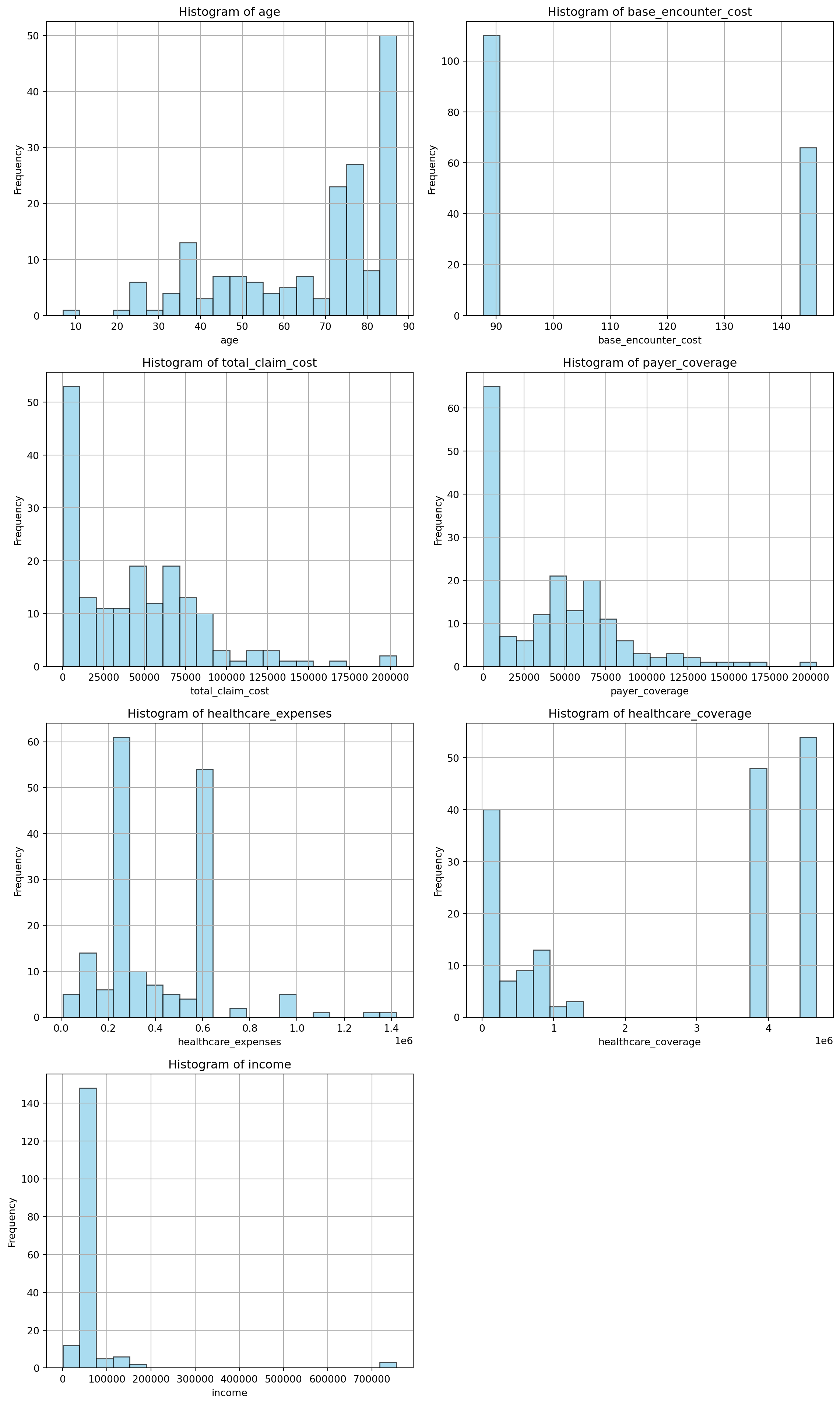
11.0.4.4 Check for class imbalance
# Check the distribution of the 'readmitted' column
readmitted_counts = df_f['readmitted'].value_counts()
print("Readmitted Counts:\n", readmitted_counts)
# Plot the distribution
plt.figure(figsize=(8, 5))
sns.countplot(x='readmitted', data=df_f, palette='Set2')
plt.title('Distribution of Readmission')
plt.xlabel('Readmitted')
plt.ylabel('Count')
plt.xticks(ticks=[0, 1], labels=['Not Readmitted', 'Readmitted'])
plt.show()
Readmitted Counts:
readmitted
False 126
True 50
Name: count, dtype: int64/var/folders/cx/3wbhcqyd3cld6gvk_xjkvr_40000gn/T/ipykernel_13342/1914624710.py:6: FutureWarning:
Passing `palette` without assigning `hue` is deprecated and will be removed in v0.14.0. Assign the `x` variable to `hue` and set `legend=False` for the same effect.
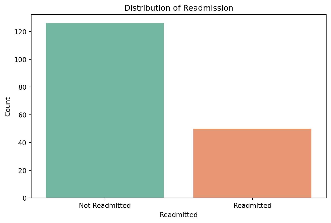
11.0.4.5 Handle class imbalance
from sklearn.utils import resample
# Separate majority and minority classes
df_majority = df_f[df_f['readmitted'] == 0]
df_minority = df_f[df_f['readmitted'] == 1]
# Upsample minority class
df_minority_upsampled = resample(df_minority,
                                  replace=True,     # sample with replacement
                                  n_samples=len(df_majority),    # to match majority class
                                  random_state=42) # reproducible results
# Combine majority class with upsampled minority class
df_f = pd.concat([df_majority, df_minority_upsampled])
# Shuffle the dataset
df_f = df_f.sample(frac=1, random_state=42).reset_index(drop=True)
# Check the new class distribution
print("New Readmitted Counts:\n", df_f['readmitted'].value_counts())
New Readmitted Counts:
readmitted
True 126
False 126
Name: count, dtype: int6411.0.5 Build Decision Tree model
from sklearn.model_selection import train_test_split
from sklearn.tree import DecisionTreeClassifier
from sklearn.metrics import classification_report, confusion_matrix, accuracy_score
import pandas as pd

# Prepare the data
X = df_f.drop(columns=['readmitted'])
X = pd.get_dummies(X, drop_first=True)  # Encode categorical variables
y = df_f['readmitted']

# Split the data
X_train, X_test, y_train, y_test = train_test_split(
    X, y, test_size=0.3, random_state=42
)

# Train a Decision Tree Classifier
dt_model = DecisionTreeClassifier(max_depth=5, random_state=42)  # You can tune max_depth
dt_model.fit(X_train, y_train)

# Make predictions
y_pred = dt_model.predict(X_test)

# Evaluate the model
print("Confusion Matrix:\n", confusion_matrix(y_test, y_pred))
print("\nClassification Report:\n", classification_report(y_test, y_pred))
print("Accuracy Score:", accuracy_score(y_test, y_pred))
Confusion Matrix:
[[37 5]
[ 5 29]]
Classification Report:
precision recall f1-score support
False 0.88 0.88 0.88 42
True 0.85 0.85 0.85 34
accuracy 0.87 76
macro avg 0.87 0.87 0.87 76
weighted avg 0.87 0.87 0.87 76
Accuracy Score: 0.86842105263157911.0.5.1 Hyperparameter Tuning for Decision Tree Classifier
from sklearn.model_selection import GridSearchCV
from sklearn.tree import DecisionTreeClassifier
from sklearn.metrics import classification_report, confusion_matrix, accuracy_score
# Prepare the data
X = df_f.drop(columns=['readmitted'])
X = pd.get_dummies(X, drop_first=True)
y = df_f['readmitted']
# Split the data
X_train, X_test, y_train, y_test = train_test_split(
X, y, test_size=0.3, random_state=42
)
# Define parameter grid
param_grid = {
'max_depth': [3, 5, 10, None],
'min_samples_split': [2, 5, 10],
'min_samples_leaf': [1, 2, 4],
'criterion': ['gini', 'entropy']
}
# Grid search with cross-validation
grid_search = GridSearchCV(
estimator=DecisionTreeClassifier(random_state=42),
param_grid=param_grid,
cv=5,
scoring='accuracy',
n_jobs=-1
)
grid_search.fit(X_train, y_train)
# Train with best estimator
best_dt_model = grid_search.best_estimator_
y_pred = best_dt_model.predict(X_test)
# Evaluate
print("Best Parameters:", grid_search.best_params_)
print("\nConfusion Matrix:\n", confusion_matrix(y_test, y_pred))
print("\nClassification Report:\n", classification_report(y_test, y_pred))
print("Accuracy Score:", accuracy_score(y_test, y_pred))Best Parameters: {'criterion': 'gini', 'max_depth': 5, 'min_samples_leaf': 1, 'min_samples_split': 2}
Confusion Matrix:
 [[37  5]
 [ 5 29]]

Classification Report:
               precision    recall  f1-score   support

       False       0.88      0.88      0.88        42
        True       0.85      0.85      0.85        34

    accuracy                           0.87        76
   macro avg       0.87      0.87      0.87        76
weighted avg       0.87      0.87      0.87        76

Accuracy Score: 0.86842105263157911.0.6 Building a Random Forest Classifier model.
from sklearn.model_selection import train_test_split
from sklearn.ensemble import RandomForestClassifier
from sklearn.metrics import classification_report, confusion_matrix, accuracy_score

# Ensure all features are numeric
X = df_f.drop(columns=['readmitted'])
X = pd.get_dummies(X, drop_first=True)  # Encode any categorical variables
y = df_f['readmitted']

# Split data
X_train, X_test, y_train, y_test = train_test_split(
    X, y, test_size=0.3, random_state=42
)

# Train Random Forest model
model = RandomForestClassifier(n_estimators=100, random_state=42)
model.fit(X_train, y_train)

# Make predictions
y_pred = model.predict(X_test)

# Evaluate the model
print("Confusion Matrix:\n", confusion_matrix(y_test, y_pred))
print("\nClassification Report:\n", classification_report(y_test, y_pred))
print("Accuracy Score:", round(accuracy_score(y_test, y_pred), 3))
Confusion Matrix:
[[36 6]
[ 3 31]]
Classification Report:
precision recall f1-score support
False 0.92 0.86 0.89 42
True 0.84 0.91 0.87 34
accuracy 0.88 76
macro avg 0.88 0.88 0.88 76
weighted avg 0.88 0.88 0.88 76
Accuracy Score: 0.88211.0.6.1 Evaluate performance of Random Forest Classifier
import matplotlib.pyplot as plt
import seaborn as sns
from sklearn.metrics import confusion_matrix

# Compute confusion matrix
cm = confusion_matrix(y_test, y_pred, labels=[False, True])

# Plot
plt.figure(figsize=(6, 5))
sns.heatmap(cm, annot=True, fmt='d', cmap='Blues', xticklabels=['Not Readmitted', 'Readmitted'], yticklabels=['Not Readmitted', 'Readmitted'])
plt.xlabel('Predicted Label')
plt.ylabel('True Label')
plt.title('Confusion Matrix')
plt.tight_layout()
plt.show()
from sklearn.metrics import classification_report
import pandas as pd

# Convert classification report to DataFrame
report = classification_report(y_test, y_pred, output_dict=True)
report_df = pd.DataFrame(report).transpose()

# Drop 'accuracy' row (optional)
report_df = report_df.drop(['accuracy'], errors='ignore')

# Plot heatmap
plt.figure(figsize=(8, 5))
sns.heatmap(report_df.iloc[:2, :3], annot=True, cmap='Greens', fmt=".2f")
plt.title('Classification Report (Precision, Recall, F1-score)')
plt.show()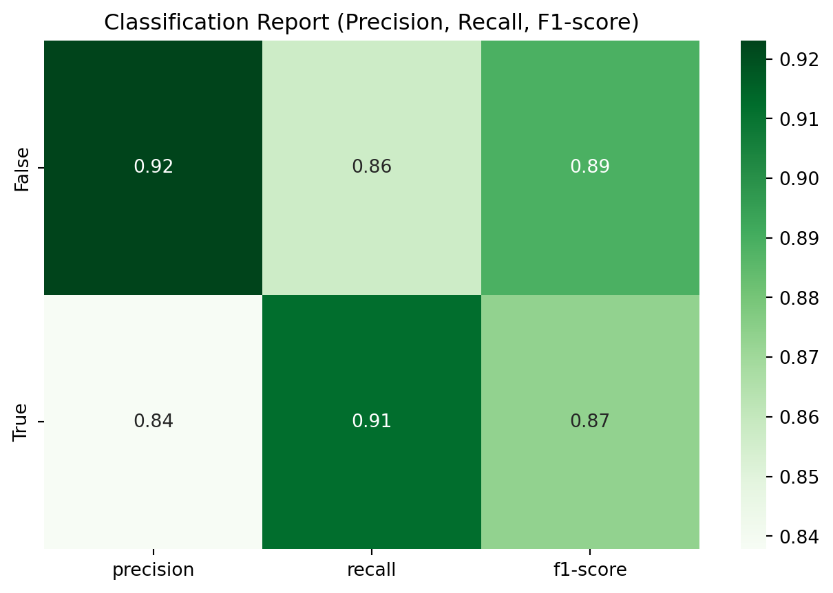
11.0.7 Building a Support Vector Machine (SVM) Classifier model
from sklearn.model_selection import train_test_split
from sklearn.svm import SVC
from sklearn.metrics import classification_report, confusion_matrix, accuracy_score
# Prepare the data
X = df_f.drop(columns=['readmitted'])
X = pd.get_dummies(X, drop_first=True)  # Encode categorical variables
y = df_f['readmitted']
# Split the data
X_train, X_test, y_train, y_test = train_test_split(
    X, y, test_size=0.3, random_state=42
)
# Train SVM model
svm_model = SVC(kernel='linear', random_state=42)  # You can also try 'rbf' or 'poly'
svm_model.fit(X_train, y_train)
# Make predictions
y_pred = svm_model.predict(X_test)
# Evaluate the model
print("Confusion Matrix:\n", confusion_matrix(y_test, y_pred))
print("\nClassification Report:\n", classification_report(y_test, y_pred))
print("Accuracy Score:", accuracy_score(y_test, y_pred))
Confusion Matrix:
[[35 7]
[ 5 29]]
Classification Report:
precision recall f1-score support
False 0.88 0.83 0.85 42
True 0.81 0.85 0.83 34
accuracy 0.84 76
macro avg 0.84 0.84 0.84 76
weighted avg 0.84 0.84 0.84 76
Accuracy Score: 0.842105263157894711.0.7.1 Evaluate performance of SVM Classifier
# Evaluate performance of SVM Classifier
import matplotlib.pyplot as plt
import seaborn as sns
# Compute confusion matrix
cm = confusion_matrix(y_test, y_pred, labels=[False, True])
# Plot confusion matrix
plt.figure(figsize=(6, 5))
sns.heatmap(cm, annot=True, fmt='d', cmap='Blues', xticklabels=['Not Readmitted', 'Readmitted'], yticklabels=['Not Readmitted', 'Readmitted'])
plt.xlabel('Predicted Label')
plt.ylabel('True Label')
plt.title('Confusion Matrix')
plt.tight_layout()
plt.show()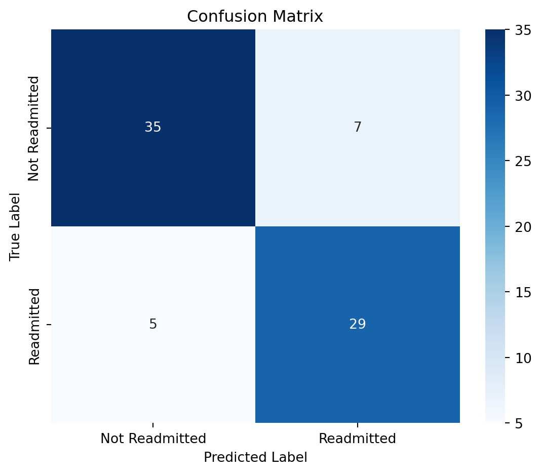
from sklearn.metrics import classification_report
# Convert classification report to DataFrame
report = classification_report(y_test, y_pred, output_dict=True)
report_df = pd.DataFrame(report).transpose()
# Drop 'accuracy' row (optional)
report_df = report_df.drop(['accuracy'], errors='ignore')
# Plot heatmap
plt.figure(figsize=(8, 5))
sns.heatmap(report_df.iloc[:2, :3], annot=True, cmap='Greens', fmt=".2f")
plt.title('Classification Report (Precision, Recall, F1-score)')
plt.show()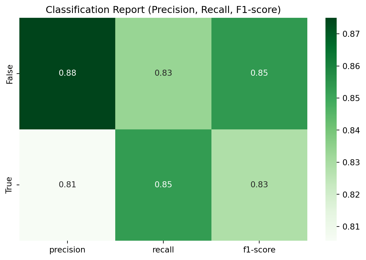
11.0.8 Building a Gradient Boosting Classifier model
from sklearn.model_selection import train_test_split
from sklearn.ensemble import GradientBoostingClassifier
from sklearn.metrics import classification_report, confusion_matrix, accuracy_score
# Prepare the data
X = df_f.drop(columns=['readmitted'])
X = pd.get_dummies(X, drop_first=True)  # Encode categorical variables
y = df_f['readmitted']
# Split the data
X_train, X_test, y_train, y_test = train_test_split(
    X, y, test_size=0.3, random_state=42
)
# Train Gradient Boosting model
gb_model = GradientBoostingClassifier(n_estimators=100, random_state=42)
gb_model.fit(X_train, y_train)
# Make predictions
y_pred = gb_model.predict(X_test)
# Evaluate the model
print("Confusion Matrix:\n", confusion_matrix(y_test, y_pred))
print("\nClassification Report:\n", classification_report(y_test, y_pred))
print("Accuracy Score:", accuracy_score(y_test, y_pred))
Confusion Matrix:
[[37 5]
[ 5 29]]
Classification Report:
precision recall f1-score support
False 0.88 0.88 0.88 42
True 0.85 0.85 0.85 34
accuracy 0.87 76
macro avg 0.87 0.87 0.87 76
weighted avg 0.87 0.87 0.87 76
Accuracy Score: 0.86842105263157911.0.8.1 Evaluate performance of Gradient Boosting Classifier
# Evaluate performance of Gradient Boosting Classifier
import matplotlib.pyplot as plt
import seaborn as sns
# Compute confusion matrix
cm = confusion_matrix(y_test, y_pred, labels=[False, True])
# Plot confusion matrix
plt.figure(figsize=(6, 5))
sns.heatmap(cm, annot=True, fmt='d', cmap='Blues', xticklabels=['Not Readmitted', 'Readmitted'], yticklabels=['Not Readmitted', 'Readmitted'])
plt.xlabel('Predicted Label')
plt.ylabel('True Label')
plt.title('Confusion Matrix')
plt.tight_layout()
plt.show()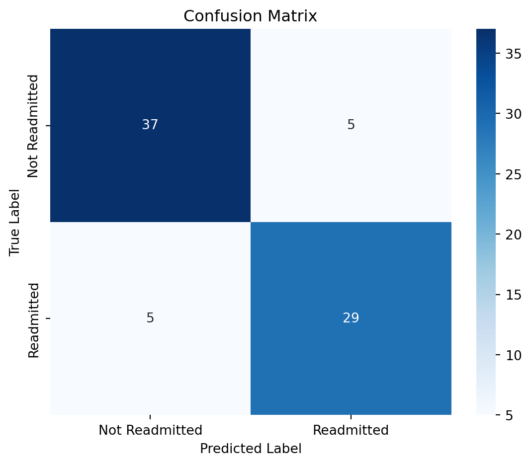
11.0.9 Conclusion
In this chapter, we explored various machine learning classification models to predict patient readmission. We started with data preprocessing, including handling missing values and encoding categorical variables. We then built and evaluated several models: Decision Tree, Random Forest, Support Vector Machine (SVM), and Gradient Boosting.
Each model was assessed based on its confusion matrix, classification report, and accuracy score. The Random Forest model generally performed well, achieving a high accuracy and balanced precision and recall. The SVM and Gradient Boosting models also showed promising results, while the Decision Tree model provided a simpler interpretation but with slightly lower performance.
The choice of model depends on the specific requirements of the healthcare setting, such as interpretability, computational resources, and the need for real-time predictions. Future work could involve hyperparameter tuning, feature selection, and exploring ensemble methods to further improve model performance.