Machine learning is a powerful tool for identifying patterns and making predictions from data, especially in healthcare. Among its many techniques, linear regression is one of the most fundamental, particularly for predicting continuous outcomes.
In this chapter, We’ll apply linear regression to a real-world healthcare dataset — heart.csv — which includes clinical and demographic data related to cholesterol levels. We’ll cover data preparation, model building, performance evaluation, and result interpretation in a medical context.
This hands-on approach reinforces core machine learning concepts and shows how even simple models can yield valuable insights. We’ll also address challenges like data missing, multicollinearity and outliers that can affect model accuracy.
10.0.2 Load python necessary packages and data
# Python packagesimport pandas as pdimport numpy as npimport seaborn as snsimport matplotlib.pyplot as plt# Load datadf= pd.read_csv("/Users/nnthieu/Downloads/heart.csv")print(df.shape)print(df.columns)df.head()
File heart.csv has 5209 rows and 17 columns, where each row represents a patient and each column represents a feature or attribute related to heart disease.
10.0.3 Evaluate the dataset
10.0.3.1 Check for missing data
The dataset contains some missing values, which we will need to handle before applying machine learning algorithms. We can check for missing values using the following code:
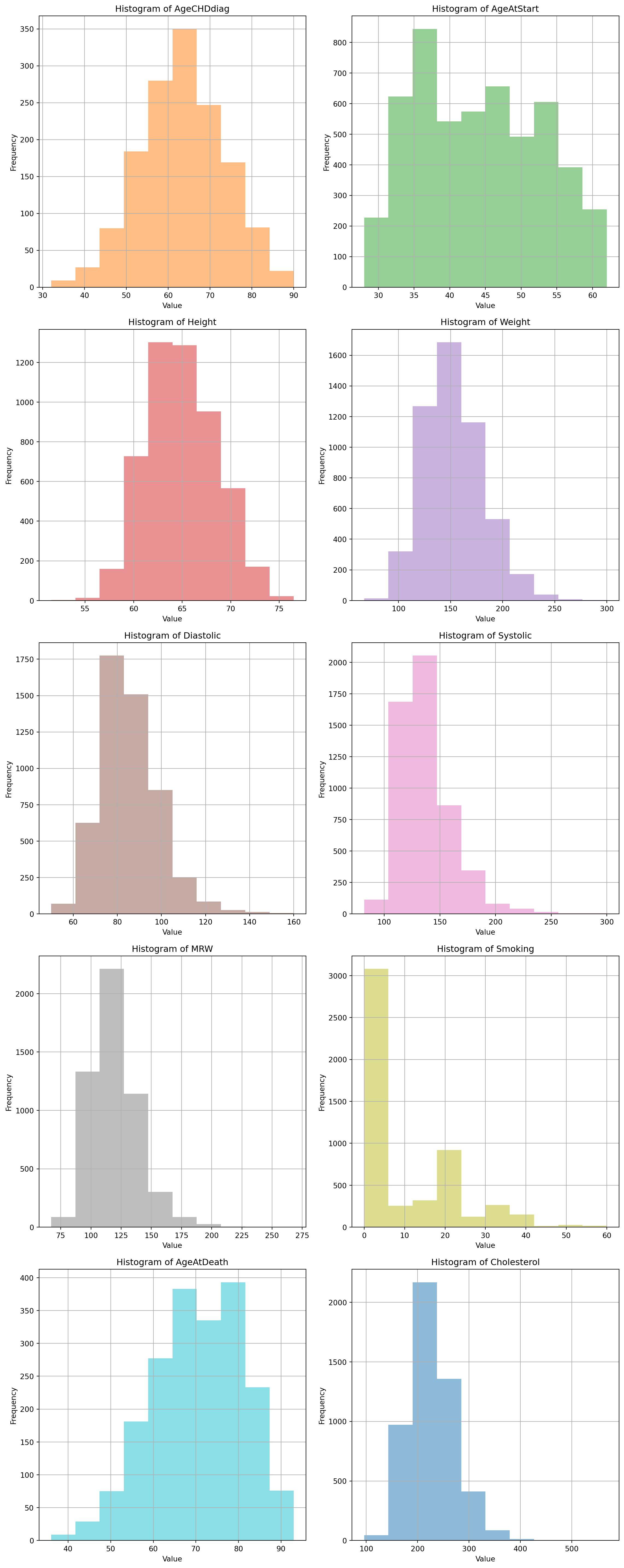
10.0.3.2 look at the data distribution of the numeric variables:
Check the histogram to see if there are any outliers in the numeric variables.
def plot_histograms(df, bins=10, alpha=0.5, colors=None):""" Plot histograms for all numeric variables in the DataFrame. Parameters: df (DataFrame): The DataFrame containing numeric variables. bins (int): Number of bins for the histograms. Default is 10. alpha (float): Transparency level of the histograms. Default is 0.5. colors (list): List of colors for the histograms. If None, default colors will be used. Returns: None """if colors isNone: colors = plt.cm.tab10.colors # Default color palette num_variables = df.select_dtypes(include='number').shape[1] num_rows = (num_variables +1) //2 num_cols =2 plt.figure(figsize=(12, 6* num_rows))for i, col inenumerate(df.select_dtypes(include='number'), start=1): plt.subplot(num_rows, num_cols, i) plt.hist(df[col], bins=bins, alpha=alpha, color=colors[i %len(colors)]) plt.title(f'Histogram of {col}') plt.xlabel('Value') plt.ylabel('Frequency') plt.grid(True) plt.tight_layout() plt.show()# Example usage:# Assuming df is your DataFrame containing numeric variablesplot_histograms(df)
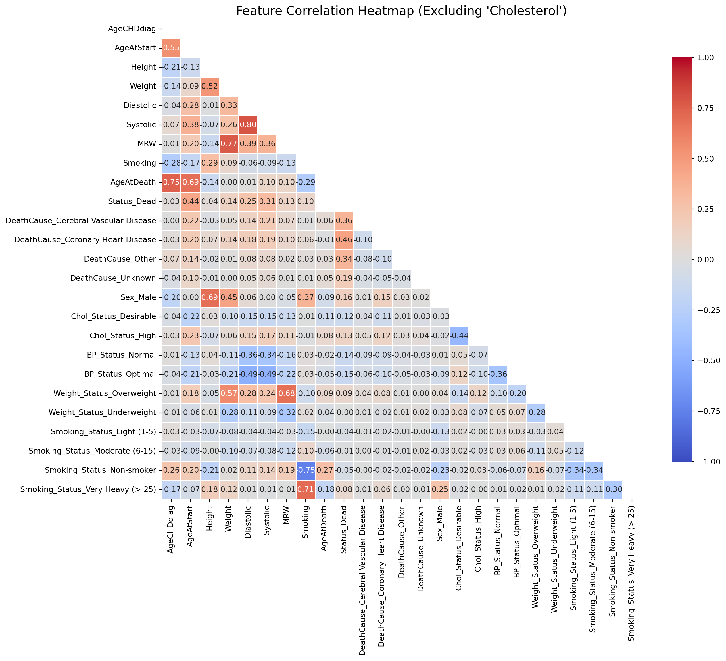
10.0.3.3 Check correlation between variables using heatmap
To visualize the correlation between variables in the dataset, We will create a heatmap. This will help us identify relationships between features and understand how they might influence cholesterol levels.
Highly correlated features can lead to multicollinearity, which can affect the performance of linear regression models. To identify pairs of features with high correlation, we will extract the upper triangle of the correlation matrix and filter for pairs with an absolute correlation greater than 0.65.
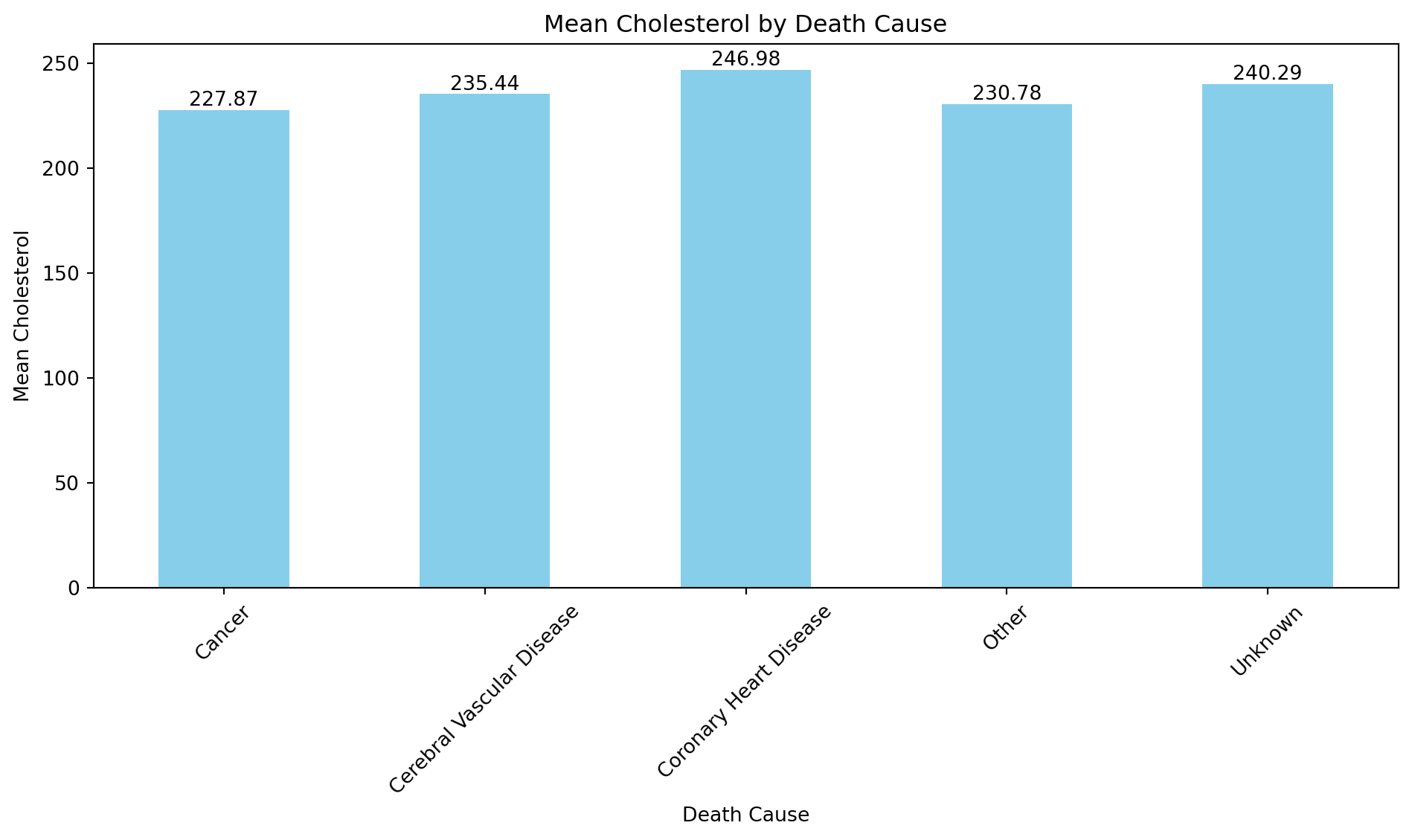
# Calculate mean cholesterol for each DeathCausemean_cholesterol = df.groupby('DeathCause')['Cholesterol'].mean()# Create bar plotplt.figure(figsize=(10, 6))mean_cholesterol.plot(kind='bar', color='skyblue')plt.title('Mean Cholesterol by Death Cause')plt.xlabel('Death Cause')plt.ylabel('Mean Cholesterol')plt.xticks(rotation=45) # Rotate x-axis labels for better visibility# Add mean values to the barsfor index, value inenumerate(mean_cholesterol): plt.text(index, value, str(round(value, 2)), ha='center', va='bottom')plt.tight_layout()plt.show()
‘DeathCause’ is consequences, not exposurer, that should be removed from the regression models.
Highly correlated features will be removed from the dataset to avoid multicollinearity issues. Therefore, we should get out variables as ‘MRW’, ‘Weight_Status_Overweight’, ‘Height’.
Data have to be prepared before applying machine learning algorithms. This includes handling missing values, recoding categorical variables, and detecting outliers.
# Calculate means for numeric columnsmeans = df.mean(numeric_only=True)# Impute missing values in numeric columns using their respective meansfor col in df.select_dtypes(include='number'): df[col] = df[col].fillna(means[col])df.describe()
AgeCHDdiag
AgeAtStart
Weight
Diastolic
Smoking
Cholesterol
count
5209.000000
5209.000000
5209.000000
5209.000000
5209.000000
5209.000000
mean
63.302968
44.068727
153.086681
85.358610
9.366518
227.417441
std
5.282496
8.574954
28.898765
12.973091
11.989796
44.274927
min
32.000000
28.000000
67.000000
50.000000
0.000000
96.000000
25%
63.302968
37.000000
132.000000
76.000000
0.000000
197.000000
50%
63.302968
43.000000
150.000000
84.000000
1.000000
225.000000
75%
63.302968
51.000000
172.000000
92.000000
20.000000
251.000000
max
90.000000
62.000000
300.000000
160.000000
60.000000
568.000000
Check NA again
df.isna().sum()
Status         0
AgeCHDdiag     0
Sex            0
AgeAtStart     0
Weight         0
Diastolic      0
Smoking        0
Cholesterol    0
Chol_Status    0
dtype: int64
10.0.4.3 Recoding data
To prepare the dataset for machine learning, we need to recode categorical variables into numerical values. This is essential because most machine learning algorithms require numerical input.
# Drop outliers from dffor col, outliers in outliers_dict.items():try: df.drop(outliers.index, inplace=True)exceptKeyError:# Handle KeyError if the column doesn't exist in the DataFramepass# Reset index after dropping outliersdf.reset_index(drop=True, inplace=True)# Verify the DataFrame after dropping outliersprint(df.head(10))
10.0.5.3 rewrite the model with top 7 variables most contribute to the model
# Encode categorical features# Identify categorical columns (object or category types)categorical_cols = df.select_dtypes(include=['object', 'category']).columns.tolist()# Optional: drop target-related columns before encodingcategorical_cols = [col for col in categorical_cols if col notin ['Cholesterol', 'Chol_Status']]# One-hot encodedf_encoded = pd.get_dummies(df, columns=categorical_cols, drop_first=True)# Split data X = df_encoded.drop(['Cholesterol', 'Chol_Status'], axis=1)y = df_encoded['Cholesterol']# Train-test splitX_train, X_test, y_train, y_test = train_test_split( X, y, test_size=0.2, random_state=42)# Initialize linear regression modelmodel = LinearRegression()# Fit the model on the training datamodel.fit(X_train, y_train)# Extract coefficientscoefficients = model.coef_# Match coefficients with feature namesfeature_names = X.columnscoefficients_df = pd.DataFrame({'Feature': feature_names, 'Coefficient': coefficients})# Sort coefficients by absolute valuecoefficients_df['Absolute Coefficient'] = coefficients_df['Coefficient'].abs()sorted_coefficients_df = coefficients_df.sort_values(by='Absolute Coefficient', ascending=False)# Select top 10 featurestop_features = sorted_coefficients_df.iloc[:7]['Feature'].tolist()# Fit the model on training data with top 10 featuresX_train_top = X_train[top_features]model.fit(X_train_top, y_train)# Evaluate the model on testing dataX_test_top = X_test[top_features]score = model.score(X_test_top, y_test)print("R-squared (R2) score using top 7 features:", score)
R-squared (R2) score using top 7 features: 0.06813581733633045
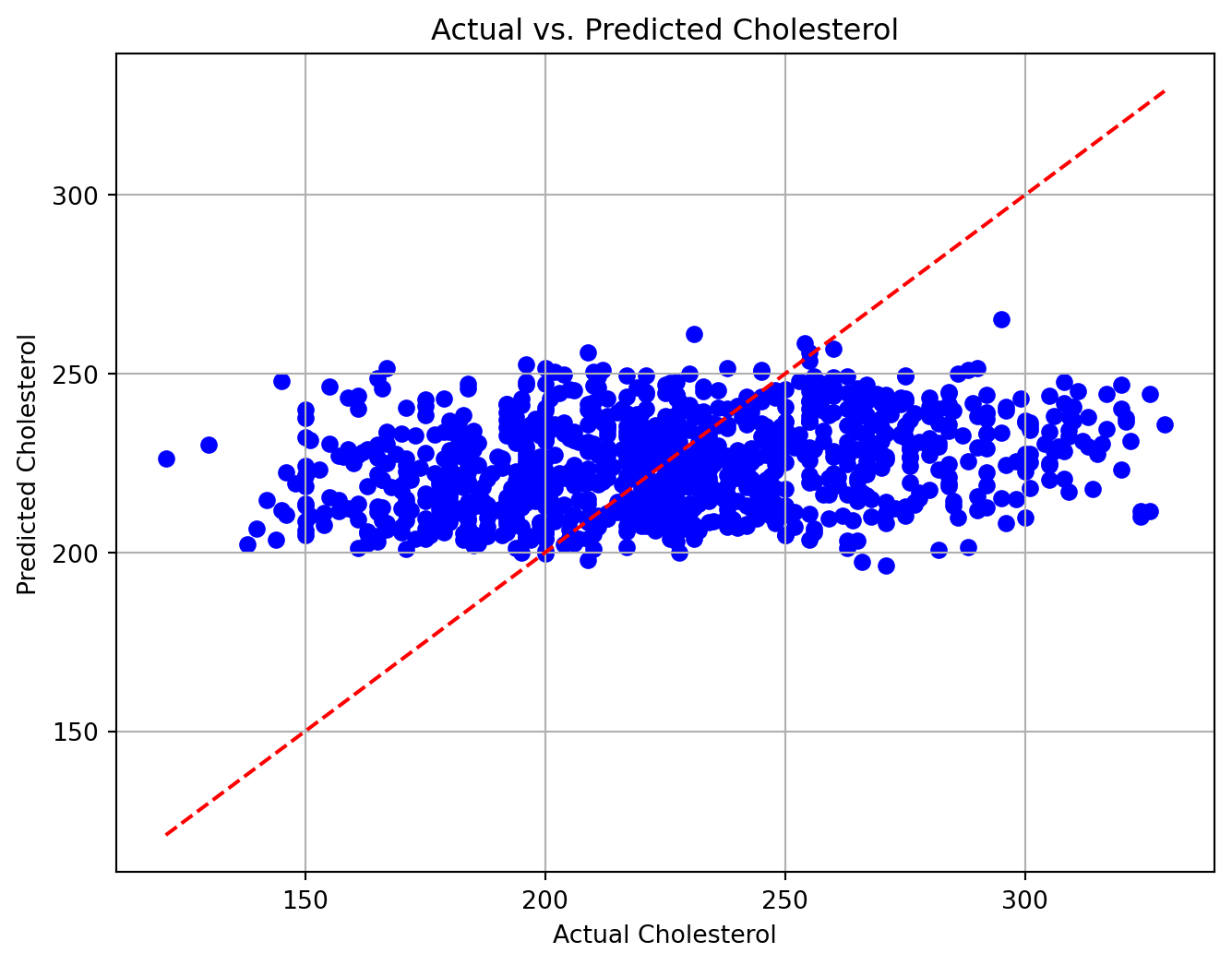
10.0.5.4 Visualization
import seaborn as snsimport matplotlib.pyplot as plt#Plot actual vs. predicted cholesterol valuesplt.figure(figsize=(8, 6))plt.scatter(y_test, y_pred, color='blue')plt.plot([min(y_test), max(y_test)], [min(y_test), max(y_test)], color='red', linestyle='--')plt.xlabel('Actual Cholesterol')plt.ylabel('Predicted Cholesterol')plt.title('Actual vs. Predicted Cholesterol')plt.grid(True)plt.show()
This is a relatively low R² score, suggesting that while the model captures some relationship between the features and cholesterol levels, there are likely other factors not included in the model that significantly influence cholesterol levels. Further feature engineering or inclusion of additional relevant variables may improve the model’s performance.
10.0.6 Running linear regression using statsmodels
import pandas as pdimport numpy as npimport statsmodels.api as smfrom sklearn.model_selection import train_test_split# Encode categorical features (skip target columns)categorical_cols = df.select_dtypes(include=['object', 'category']).columns.tolist()categorical_cols = [col for col in categorical_cols if col notin ['Cholesterol', 'Chol_Status']]df_encoded = pd.get_dummies(df, columns=categorical_cols, drop_first=True)# Define features and targetX = df_encoded.drop(['Cholesterol', 'Chol_Status'], axis=1)y = df_encoded['Cholesterol']# Step 3: Split into train/test setsX_train, X_test, y_train, y_test = train_test_split( X, y, test_size=0.2, random_state=42)# Align test columns to trainX_train, X_test = X_train.align(X_test, join='left', axis=1, fill_value=0)# Ensure all data is numeric and float (important for statsmodels)X_train = X_train.astype(float)X_test = X_test.astype(float)y_train = y_train.astype(float)# Add constant for interceptX_train = sm.add_constant(X_train)X_test = sm.add_constant(X_test)# Fit the modellm2 = sm.OLS(y_train, X_train).fit()# Show summaryprint(lm2.summary())
                            OLS Regression Results
==============================================================================
Dep. Variable:            Cholesterol   R-squared:                       0.106
Model:                            OLS   Adj. R-squared:                  0.105
Method:                 Least Squares   F-statistic:                     68.41
Date:                Sat, 28 Jun 2025   Prob (F-statistic):           1.12e-93
Time:                        10:20:16   Log-Likelihood:                -20370.
No. Observations:                4042   AIC:                         4.076e+04
Df Residuals:                    4034   BIC:                         4.081e+04
Df Model:                           7
Covariance Type:            nonrobust
==============================================================================
                 coef    std err          t      P>|t|      [0.025      0.975]
------------------------------------------------------------------------------
const        157.0432      8.898     17.649      0.000     139.598     174.489
Status         2.0063      1.403      1.430      0.153      -0.743       4.756
AgeCHDdiag    -0.4347      0.121     -3.596      0.000      -0.672      -0.198
Sex           -6.2224      1.444     -4.310      0.000      -9.053      -3.392
AgeAtStart     1.2381      0.084     14.799      0.000       1.074       1.402
Weight         0.1088      0.026      4.239      0.000       0.058       0.159
Diastolic      0.2848      0.051      5.596      0.000       0.185       0.385
Smoking        0.1983      0.055      3.634      0.000       0.091       0.305
==============================================================================
Omnibus:                       44.661   Durbin-Watson:                   2.043
Prob(Omnibus):                  0.000   Jarque-Bera (JB):               45.040
Skew:                           0.245   Prob(JB):                     1.66e-10
Kurtosis:                       2.835   Cond. No.                     2.91e+03
==============================================================================

Notes:
[1] Standard Errors assume that the covariance matrix of the errors is correctly specified.
[2] The condition number is large, 2.91e+03. This might indicate that there are
strong multicollinearity or other numerical problems.
statsmodels improves R-squared score to 0.114.
Identify influenced rows that might affect the model performance. We will use studentized residuals to detect outliers.
# If resid was computed from statsmodels on X_train:outliers = np.abs(resid["Studentized Residuals"]) >3ind = resid[outliers].index# Only drop if the indices actually existvalid_ind = [i for i in ind if i in X_train.index]X_train.drop(index=valid_ind, inplace=True)y_train.drop(index=valid_ind, inplace=True)
10.0.6.1 Detecting and removing multicollinearity
Multicollinearity occurs when two or more independent variables in a regression model are highly correlated, which can lead to unreliable coefficient estimates. We can detect multicollinearity using the Variance Inflation Factor (VIF).
from statsmodels.stats.outliers_influence import variance_inflation_factor[variance_inflation_factor(X_train.values, j) for j inrange(X_train.shape[1])]
We create a function to remove the collinear variables. We choose a threshold of 5 which means if VIF is more than 5 for a particular variable then that variable will be removed.
def calculate_vif(x): thresh =5.0 output = pd.DataFrame() k = x.shape[1] vif = [variance_inflation_factor(x.values, j) for j inrange(x.shape[1])]for i inrange(1,k):print("Iteration no.")print(i)print(vif) a = np.argmax(vif)print("Max VIF is for variable no.:")print(a)if vif[a] <= thresh :breakif i ==1 : output = x.drop(x.columns[a], axis =1) vif = [variance_inflation_factor(output.values, j) for j inrange(output.shape[1])]elif i >1 : output = output.drop(output.columns[a],axis =1) vif = [variance_inflation_factor(output.values, j) for j inrange(output.shape[1])]return(output)train_out = calculate_vif(X_train)train_out.head(3)
Iteration no.
1
[228.80071850018703,
 1.3394416883894844,
 1.1289095898066266,
 1.491372090282602,
 1.4737894670530807,
 1.421536015030276,
 1.247273518820798,
 1.2456096632455371]
Max VIF is for variable no.:
0
Iteration no.
2
[2.1222882889369488, 62.16034485702503, 2.701296037094943, 40.41113912383457, 42.09374206836035, 49.06828510997345, 1.920379036703248]
Max VIF is for variable no.:
1
Iteration no.
3
[1.9248923624254433, 2.6206724232173713, 28.190316957166747, 37.075574349814076, 42.868450858747245, 1.8715880307447514]
Max VIF is for variable no.:
4
Iteration no.
4
[1.9248781994016138, 2.5134621648001754, 20.368687501825814, 22.04762828608679, 1.8584351804464543]
Max VIF is for variable no.:
3
Iteration no.
5
[1.8435708145893481, 2.136544517299741, 2.5600136791453187, 1.8168711072464279]
Max VIF is for variable no.:
2
Status
Sex
AgeAtStart
Smoking
4942
1.0
0.0
49.0
0.0
2833
0.0
1.0
36.0
30.0
1041
0.0
0.0
52.0
0.0
10.0.6.2 Running linear regression again on our new training set (without multicollinearity)
import pandas as pdimport numpy as npimport statsmodels.api as smfrom sklearn.model_selection import train_test_split# Encode categorical features (skip target columns)categorical_cols = df.select_dtypes(include=['object', 'category']).columns.tolist()categorical_cols = [col for col in categorical_cols if col notin ['Cholesterol', 'Chol_Status']]df_encoded = pd.get_dummies(df, columns=categorical_cols, drop_first=True)# Step 2: Define features and targetX = df_encoded.drop(['Cholesterol', 'Chol_Status'], axis=1)y = df_encoded['Cholesterol']# Split into train/test setsX_train, X_test, y_train, y_test = train_test_split( X, y, test_size=0.2, random_state=42)# Step 4: Align test columns to trainX_train, X_test = X_train.align(X_test, join='left', axis=1, fill_value=0)# Ensure all data is numeric and float (important for statsmodels)X_train = X_train.astype(float)X_test = X_test.astype(float)y_train = y_train.astype(float)# Add constant for intercepttrain_out = sm.add_constant(train_out)X_test = sm.add_constant(X_test)# Step 7: Fit the modellm2 = sm.OLS(y_train, X_train).fit()# Show summaryprint(lm2.summary())
                                 OLS Regression Results
=======================================================================================
Dep. Variable:            Cholesterol   R-squared (uncentered):                   0.971
Model:                            OLS   Adj. R-squared (uncentered):              0.971
Method:                 Least Squares   F-statistic:                          1.935e+04
Date:                Sat, 28 Jun 2025   Prob (F-statistic):                        0.00
Time:                        10:20:20   Log-Likelihood:                         -20520.
No. Observations:                4042   AIC:                                  4.105e+04
Df Residuals:                    4035   BIC:                                  4.110e+04
Df Model:                           7
Covariance Type:            nonrobust
==============================================================================
                 coef    std err          t      P>|t|      [0.025      0.975]
------------------------------------------------------------------------------
Status        -1.2945      1.442     -0.897      0.370      -4.123       1.534
AgeCHDdiag     1.2664      0.076     16.726      0.000       1.118       1.415
Sex           -8.0096      1.494     -5.360      0.000     -10.940      -5.080
AgeAtStart     1.3199      0.087     15.227      0.000       1.150       1.490
Weight         0.2334      0.026      9.114      0.000       0.183       0.284
Diastolic      0.5905      0.050     11.891      0.000       0.493       0.688
Smoking        0.4139      0.055      7.500      0.000       0.306       0.522
==============================================================================
Omnibus:                       37.541   Durbin-Watson:                   2.037
Prob(Omnibus):                  0.000   Jarque-Bera (JB):               38.476
Skew:                           0.238   Prob(JB):                     4.42e-09
Kurtosis:                       2.949   Cond. No.                         486.
==============================================================================

Notes:
[1] R² is computed without centering (uncentered) since the model does not contain a constant.
[2] Standard Errors assume that the covariance matrix of the errors is correctly specified.
R-squared score is improved significantly to 0.971 and no more multicolinear variables.
10.0.7 Conclusion
In this chapter, we explored the application of linear regression to a healthcare dataset, specifically focusing on predicting cholesterol levels. We demonstrated the importance of data preparation, including handling missing values, encoding categorical variables, and detecting outliers. We also addressed multicollinearity by calculating Variance Inflation Factor (VIF) and removing collinear variables, which significantly improved the model’s performance.
We built a linear regression model using the statsmodels library, which provided detailed insights into the model’s performance and the significance of each feature. The final model achieved a high R-squared score, indicating that it explained a substantial portion of the variance in cholesterol levels.